Overview

The checkerboard pattern is a classic example of a procedural texture — generated entirely by the GPU at runtime without any image data. No texture atlas, no sprite: just math executed in the fragment shader for every pixel on screen.

In this article, we'll build the algorithm step by step, introducing several mathematical concepts through GLSL functions that make repetition possible — fract(), floor(), and mod() — and illustrating how they fit together to produce the alternating grid effect. From there we'll extend the pattern with colors, add animation to the grid, and explore a more hardware-friendly optimization of the algorithm.

Pixels & Coordinates

The fragment shader runs once per pixel, and each one carries its own position in screen space. That position is all we need to start generating patterns — no textures, no external data, just math evaluated at every single point on screen.

UV Coordinates

---

To start manipulating each pixel individually, we'll work with UV coordinates — a 2D vector directly tied to each pixel's position on screen. These coordinates are normalized meaning both components range from 0.0 to 1.0 across the entire surface and provide a continuous coordinate space where each pixel receives a distinct interpolated value. This allows us to achieve smooth effects and transformations.

The U component increases left → right, while V increases bottom → top (following OpenGL convention). As a result, any mathematical operation applied to the UVs directly affects how the pattern is distributed across the surface.

Solid Color

---

As a starting point, we can directly ignore UV coordinates and just output a constant color. Thus, every pixel ends up with vec4(R, G, B, A).

Code

Visualization

Solid color output — every pixel is identical

UV Color

---

Now let's use the provided UVs as the color output for each pixel. By mapping U → Red and V → Green we can quickly verify that the coordinate system is working correctly before applying the actual pattern.

Code

Reading the four corners:

• Bottom-left → black (UV = 0, 0)
• Bottom-right → red (UV = 1, 0)
• Top-left → green (UV = 0, 1)
• Top-right → yellow (UV = 1, 1)

Visualization

UV coordinates as color (R = U, G = V)

Repetition Techniques

Now that each pixel has a well-defined position in UV space, we can begin shaping those coordinates to create repeating patterns with the following techniques.

UV Scaling

---

The first step toward any tiled pattern is scaling. By multiplying the UV coordinates by a scalar, we spread them over a larger range. Multiplying by N expands the coordinates to a range of [0, N], effectively creating an N × N grid. For example, with a scale of 4, the U component runs from 0 to 4 across the surface instead of 0 to 1.

The issue arises when color values exceed 1.0. GPUs clamp all channels to the [0, 1]. range, so any excess saturates to white. As a result, a scaled gradient floods with maximum color. The underlying pattern is still present mathematically, but it’s compressed beyond what the display can show, leaving a flat, washed-out image.

Code

Visualization

UV × scale — values above 1.0 clamp to white (saturated)

Increase the scale and notice how the right and top portions flood with solid color. Since multiplying UVs can push them beyond 0–1, we need a way to wrap them back. The GLSL function fract() handles this perfectly, keeping every value within the normalized range.

fract(x) returns the fractional part of a number: fract(x) = x − floor(x) For any value, it discards the integer part and keeps only the decimal component. This effectively wraps the range [0, ∞) back into [0, 1), repeating the same interval over and over.

Applying fract() after scaling wraps every tile's coordinates back into [0, 1], making the gradient repeat identically across each cell.

Code

Visualization

fract(UV × scale) — the gradient now tiles perfectly

UV Flooring & Normalization

---

While fract() is a valid way to produce repetition, the approach we'll use for the checkerboard relies on floor() instead.

floor(x) rounds a number down to the nearest integer (⌊x⌋). ⌊x⌋ = largest integer n where n ≤ x This operation is commonly used to extract the integer portion of a value, allowing continuous values to be converted into discrete intervals. This makes it useful for identifying and indexing grid cells in procedural algorithms.

By rounding down the scaled UV coordinates, it produces a range of cell indices from (0,0) at the bottom-left to (N,N) at the top-right, as defined by the following expression:

Since these values exceed 1.0, we normalize them back into the [0,1] range by dividing by the same scale factor. This makes each cell’s unique index visible as a discrete color step.

Code

Visualization

floor(UV × scale) / scale — each cell is a flat, uniform color

Note that the output colors appear slightly darker than usual. This is expected, since the normalized values never reach 1.0 — the largest cell index always will be uScale - 1.

Every pixel within the same cell shares an identical cellIndex, so they all produce the same output. Thus, forming the basis of discrete cell-based repetition patterns.

Modulo Operation

---

So far, so good but now we need something to flip between two states — black and white — as we move from one cell to the next. The modulo operation mod() gives us exactly that: a way to alternate between 0 and 1 with every step.

mod(x, y) returns the remainder of x divided by y, defined as: x − y · floor(x / y) For integer inputs with a divisor of 2, the result is 0 for even numbers and 1 for odd numbers — producing a simple binary alternation.

Applying mod(cellIndex, 2.0) to the integer cell indices, we get a strict 0/1 alternation, as it flips the value with every step from one cell to the next:

x (cell index)	mod(x, 2)	Parity
0	0	EVEN
1	1	ODD
2	0	EVEN
3	1	ODD

If we apply the modulo only to the X component of the cell index, the Y axis is ignored entirely. Every column alternates between black (0) and white (1), but all rows within a column are identical — producing vertical stripes.

Code

Visualization

mod(floor(U × scale), 2.0) — vertical stripes (Y ignored)

XOR

---

To get a checkerboard instead of stripes, both axes must contribute. The logical operation that connects them is XOR (exclusive or): two cells should have opposite colors when their X and Y parities differ, and the same color when they match.

XOR (A ⊕ B) (eXclusive OR) is a logic operation that returns 1 only when its two inputs differ, and 0 when they are equal. The formal Boolean definition is as follows: A ⊕ B = (A ∧ ¬B) ∨ (¬A ∧ B) A and B follow this condition: either A is true and B is false, or A is false and B is true; not both.

When working with single-bit values, XOR can be expressed using basic arithmetic. In practice, this means we can calculate XOR with ordinary addition and modulo operations, without any bitwise instructions needed.

The arithmetic expression is defined as follows:

So summing the two cell indices and taking mod 2 is mathematically identical to XOR-ing their parities:

A (cellX parity)	B (cellY parity)	(A + B) mod 2	A XOR B
0	0	0	0
0	1	1	1
1	0	1	1
1	1	0	0

As the table shows, The columns (A + B) mod 2 and A XOR B are always equal. This demostrates that mod(cellX + cellY, 2.0) correctly produces the alternating pattern of a checkerboard..

To visualize this geometrically, here is a 4×4 grid of cells with their coordinates and pre-mod sums. Even sums (0, 2, 4, 6…) yield one color; odd sums (1, 3, 5…) yield the other:

Code

Visualization

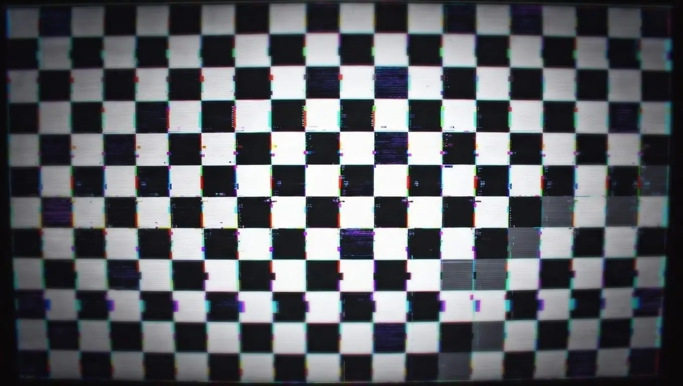
mod(floor(U × s) + floor(V × s), 2.0) — the classic checkerboard

Variations & Enhancements

Now that we have the core pattern working, the black-and-white grid is just the starting point. With just a few additional lines of code, we can enhance the effect with custom colors, animation over time, aspect ratio adjustments to keep square cells, and much more. Let's jump into some of them!

Colored Checkerboard

---

As we've seen, the checker value alternates between 0 and 1, making it a natural fit for mix(). This allows us to blend between any two colors instead of just black and white.

mix(a, b, t) performs a linear interpolation between two values. When t = 0 it returns a, when t = 1 it returns b, and anything in between blends them proportionally: mix(a, b, t) = a · (1 − t) + b · t In GLSL it works component-wise on vectors, making it ideal for blending colors.

Code

Visualization

Colored checkerboard using mix(color1, color2, checker)

Animated Checkerboard

---

Adding motion is really straightforward. We introduce a uTime uniform (seconds elapsed since start) and use it to offset the UV coordinates before computing the cell index. This simple pattern UV + offset is a common technique in shader programming for applying movement to textures and procedural patterns.

Code

Visualization

Animated checkerboard — the offset drifts with uTime

Optimization

The mod() function works correctly, but on many GPU architectures it is implemented as a multi-instruction sequence (it compiles to a divide, a floor, a multiply, and a subtract). Since shaders run on millions of pixels every frame, replacing it with more ALU-efficient arithmetic operations can improve performance.

ALU (Arithmetic Logic Unit) is the component of the GPU responsible for executing mathematical and logical operations, including additions, multiplications, comparisons, and so on. Each shader instruction maps to one or more ALU operations, and since fragment shaders run once per pixel, reducing the ALU cost of a single instruction directly scales across the entire screen.

The trick is to use dot(), fract(), and step() together to produce the same 0/1 alternation:

dot(a, b) computes the dot product of two vectors which is the sum of the products of their corresponding components: dot(a, b) = a.x · b.x + a.y · b.y

Applied to dot(cellIndex, vec2(0.5)), this is arithmetically equivalent to:

Breaking it down step by step:

• dot(cellIndex, vec2(0.5)) computes (X × 0.5 + Y × 0.5) which is equivalent to (X + Y) × 0.5 using a single vectorized multiply-add operation.
• fract() keeps only the fractional part of the result, wrapping the value into the [0, 1) range. In this case, integers become 0.0 while half-integers remain 0.5.
• step(0.5, …) then performs the binary split and returns 1.0 if the value ≥ 0.5, otherwise 0.0.

The following table shows the equivalence for integer sums S = cellX + cellY:

S = X + Y	S × 0.5	fract(S × 0.5)	step(0.5, fract)	mod(S, 2)
0	0.0	0.0	0.0	0
1	0.5	0.5	1.0	1
2	1.0	0.0	0.0	0
3	1.5	0.5	1.0	1

The last two columns are always identical — the expressions are mathematically equivalent for integer S.

Why dot() over (X+Y)*0.5?

Both expressions produce the same result. The dot(cellIndex, vec2(0.5)) form is more idiomatic in GLSL since dot products are native operations in the GPU's vector ALU pipeline. It also reads more clearly, expressing the idea of a weighted sum instead of spelling it out as separate scalar multiplications. On modern GPUs the performance difference is usually small, but this pattern is still common in production shaders because it maps naturally to the hardware.

Code

Visualization

Optimized checkerboard — step(0.5, fract(dot(cellIndex, vec2(0.5))))

Summary

Up to this point, we've built the checkerboard by scaling the UV coordinates, snapping pixels into discrete cells with floor(), and applying mod() to the sum of the cell indices, effectively alternating between 0 and 1 like an XOR operation, to create the checkerboard pattern.

Then we add extra features like color using mix(), animation with a time-based UV offset, and making the shader more GPU-friendly by replacing mod() with a dot() + fract() + step() expression, which produces the same result at a lower ALU cost.

In short, the formulas look like this:

Standard checkerboard pattern formula

Optimized checkerboard pattern formula